EXTRAPOLATE Tab
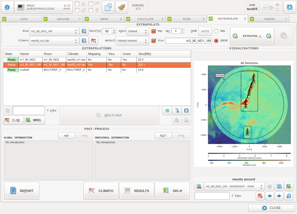
The EXTRAPOLATE Tab
The EXTRAPOLATE process applies a given climatology on previously generated rose results, so that the reference climatology can be extrapolated to the entire area of interest.
The results of EXTRAPOLATE process will be used as the inputs of ASSESS process, or exported as .wrg files to be processed in other softwares.
This process also allows considering extrapolated results from multiple met masts by combining the results.
Process options

Reference rose result and wind data
- The CFD rose results to be used to extrapolate on the projected area.
- Wind data corresponding to the CFD rose reference point.
If no corresponding data is available to use, the extrapolation may not reflect realistically the wind resource distribution.

Number of sectors
The number of sectors to use for the extrapolation’s sectorized results. The default value is set at 36, it can be modified from the User preferences.

Weibull fitting method
Defines the Weibull fitting method used in extrapolation process (cf. Weibull fitting). The default method is the Moments method, it can be modified from the User preferences.

Mapping, Visualisation features
- When Map is checked, it allows to export WRG files of the entire zone instead of points, plus the ISO-H visualizations are activated for the mapping areas.
- When Visu is checked, the ISO-H visualizations are activated for the entire projected area.
Note
These options are only available if they were activated for the selected Rose.

Reference height
This only affects the sectorization of the results: Since direction at a given location may vary with height, we have to specify which height to take into account when visualizing results by wind sectors. The default value is set at 80m, it can be modified from the User preferences.
Multi-Reference

It is possible to combine extrapolation results from multiple met masts in order to lower the uncertainty in the ASSESS process.
This process uses inverse distance weighting (distance to the reference met masts) to average the different extrapolation results, according to Shepard’s method.
- Multi-select the extrapolation results to be combined.
- Click on MULTI-REF
Note
- The extrapolation results used for multi-references are supposed to have good representation of the projected area.
- The combination cannot be repeatetd.
- The extrapolations to combine must have the same “Hvane” and “Nsect” options.
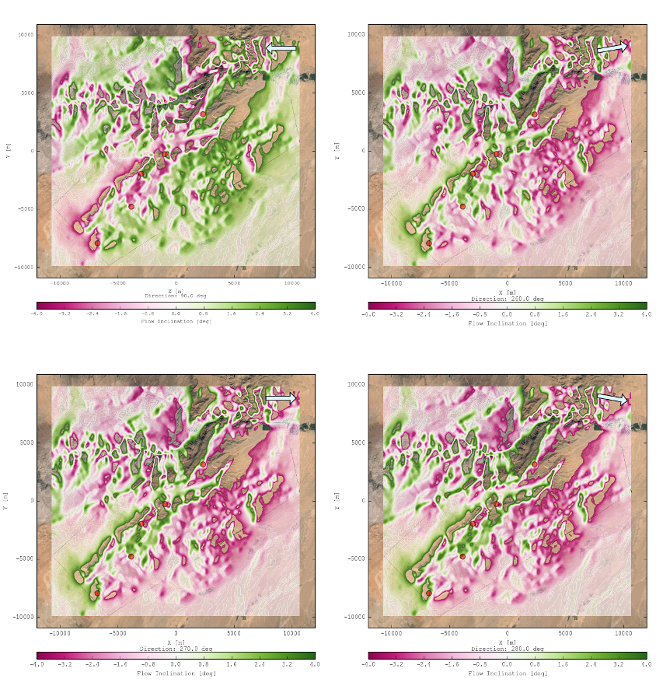
Visualizations
The EXTRAPOLATE Tab features Maps & Iso-Heights, Vertical Profiles, and Roses visualizations.
For maps and wind profiles the plottable variables are:
- Horizontal wind speed
- Flow inclination
- Turbulence intensity
- Weibull Scale Parameter - A
- Weibull Shape Parameter - K
- Wind power density (cf. Wind power density)
For wind roses the plottable variables are:
- Average wind speed
- Wind power density
- Flow inclination
- Absolute TI
- Extrapolated TI
Exportation
Climatology

This button allows to export the extrapolated wind data at each entity into tab, WRG, or zsvd/zsvds format.
Wind Resource Grid

This button allows to export gridded data files for each mapping entity into WRG or WRB format.
Note
To be able to export grid files, make sure to activate the Map option for the ROSE and EXTRAPOLATE processes.
WRG files
The conventional WRG format introduced by WAsP is a text file containing one header line, followed by one line per location considered, with the following information:
- X and Y coordinates [m]
- Terrain elevation, considered height [m]
- Weibull parameters A [m/s] and k
- Wind Power Density [W/m2]
- Number of sectors considered
Then, for each sector one after another:
- Predicted directional frequency
- Directional Weibull parameters A [m/s] and k
Warning
Although the conventional WRG format is widely used, it has significant limitations, including limited data precision and an inability to incorporate wind resource data other than the Weibull factors which do not always represent actual wind speed frequency distributions with good accuracy.
WRB files
The WRB format introduced by OpenWind is a binary file meant to address the lack of precision of WRG files. In addition to the information of a WRG file, it can include inflow angles, turbulence intensity, wind shear coefficients…
Please consult the OpenWind manual for the complete specifications of the WRB format.
Shape file
Users can control the display range of any variable results at any height above ground level and generate corresponding shape files (*.shp) for each variable.
Layout Condition Filter(Inclination angle)
Technical notes
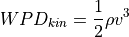
Wind power density
The formula for wind power density is usually derived from the classic wind power formula  ,
by simply normalizing it with the rotor area A, to get a density in W/m²:
,
by simply normalizing it with the rotor area A, to get a density in W/m²:
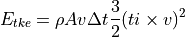
To take the Turbulent Kinetic Energy into account as well, we calculate the turbulent wind power density. The Turbulent Kinetic Energy is expressed as:
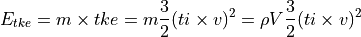
Now considering a small time  during which the air goes trhough a small volume of section A such that
  , we write:
Then dividing by time and section we get the turbulent wind power density:
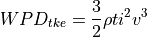
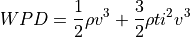
Which we add to the kinetic wind power density to get the total wind power density:
Weibull fitting
The statistical distribution most widely used to represent wind data is the 2-parameter Weibull distribution. Its Probability Density Function (PDF) and Cumulative Distribution Function (CDF) are defined as:
![f(v) = \frac{k}{A} \left(\frac{v}{A}\right)^{k-1} \exp\left[ -\left(\frac{v}{A}\right)^k \right] \\
F(v) = 1 - \exp\left[ -\left(\frac{v}{A}\right)^k \right]](../_images/math/160937637b67686ec347cc719902676ae75e97d9.png)
where 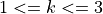 is the unitless shape parameter, and
  is the scale parameter in m/s.
To fit such a distribution from the extrapolation results, ZephyTOOLS implements 4 different methods:
- “Moments” -> Method of Moments
- “Least Squares” -> Least Squares Linear Regression
- “Max likelihood” -> Maximum Likelihood Estimation
- “Energy fitting” -> WAsP Method
Moments
The Method of Moments consists in equating the first 2 sample moments found in the data to the corresponding 2 population moments expected.
The obtained system of 2 equations allows to solve for the 2 parameters  .
.
The  population moment
  of the Weibull distribution is given by:
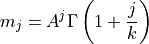
Where  is the gamma function.
The sample moment
is the gamma function.
The sample moment  of the data is computed as:
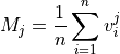
And as such,  (i.e. the data mean).
By equating
(i.e. the data mean).
By equating  and
and  we obtain the system:
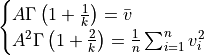
This system has no analytical solution for  and would have to be solved numerically.
ZephyTOOLS instead considers the log-transformed data, taking  .
The obtained data follows a type-I minimum distribution
(better known as minimum Gumbel distribution, or log-Weibull distribution).
Its PDF and CDF are defined as:
.
The obtained data follows a type-I minimum distribution
(better known as minimum Gumbel distribution, or log-Weibull distribution).
Its PDF and CDF are defined as:
![g(x) = \frac{1}{\beta} \exp\left[ \frac{x-\mu}{\beta} \exp \left( \frac{x-\mu}{\beta} \right) \right] \\
G(x) = 1 - \exp\left[ -\exp\left(\frac{x-\mu}{\beta}\right) \right]](../_images/math/bc79d7b7f79961ac81a4c7c8cdd0453395592af8.png)
With:

While the method of moments on the original Weibull distribution has no analytical solution,
when using the log-Weibull distribution it can give estimators for the mean  and the standard deviation
  :
:
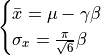
Where  is the Euler-Mascheroni constant.
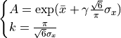
So, the Weibull parameters can be estimated with:
is the Euler-Mascheroni constant.
So, the Weibull parameters can be estimated with:
Least Squares
The Linear Least Squares regression can be used on the Weibull CDF when rearranged as:
![\ln \left[ -\ln \left(1-F(v)\right) \right] = k\ln v - k\ln A](../_images/math/5eb6fa5d50d6b6caca4f9617237efeb9c472999c.png)
Which corresponds to a linear function  with:
with:
![\begin{cases}
y = \ln \left[ -\ln \left(1-F(v)\right) \right] \\
x = \ln v
\end{cases}](../_images/math/dd43b026dd72a2251159889035436151a936f3e3.png)
Where  is known from the frequency matrix of the data.
The parameters
is known from the frequency matrix of the data.
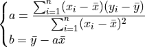
The parameters  and
and  are estimated with the Linear Least Squares regression as:
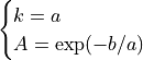
Finally the Weibull parameters are found with:
Max Likelihood
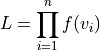
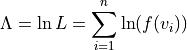
The Maximum Likelihood Estimation finds the Weibull parameters which maximize the statistical likelihood of the available data. The likelihood function is a product of the PDF functions, with one element for each data point in the data set:
It is mathematically easier to manipulate this function by first taking the logarithm of it. This log-likelihood function then has the form:
The log-likelihood function is computed for several pairs of parameters .
Initially combinations from coarse ranges of A and k values are tested, and the combination which returns the highest likelihood is taken as a first estimation.
Then the software tests iteratively several new ranges of values, each time with a finer step and always centered around the last estimation of .
This process allows to quickly assess with a precision of  for both.
Energy fitting
An implementation of WAsP’s method for Weibull fitting.
This method consists in finding the parameters which fill two conditions:
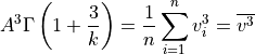
- The mean of the cubed wind speed of the fitted distribution is equal to that of the data. This comes down to equating the expected third moment to the corresponding third moment found in the data, much like what is done in the method of moments:
- The fitted distribution’s probability of winds above the data’s mean wind speed is equal to the proportion of the data meeting this requirement.
If we call this proportion
 we can express the condition as:
![1 - F(\bar{v}) = P_{v_i>\bar{v}} \\
\Leftrightarrow \exp\left[ -\left(\frac{\bar{v}}{A}\right)^k \right] = P_{v_i>\bar{v}}](../_images/math/e50746cd94ae8eebe7e8485a2276266e8620f1f8.png)
Finally,  can be subsituted using the first equation to get a single expression:
![\exp\left[ -\left( \bar{v}/\left(\frac{\overline{v^3}}{\Gamma \left(1+\frac{3}{k}\right)}\right)^{1/3} \right)^k \right] = P_{v_i>\bar{v}}](../_images/math/d78bcefdb3fddb0b0bb881de4c08db97d64a6f4a.png)
The left part of the equation is computed for several values of .
Initially a coarse range of k values is tested, from low to high until the first value allowing to meet the requirement is found.
Then the software tests iteratively several new ranges of , each time with a finer step and always centered around the last found acceptable value.
This process allows to quickly assess with a precision of .
Once is set, is calculated by solving the first condition’s equation.
IEC suitability
ZephyCFD provides all the tools to perform IEC site suitability analysis at each turbine locations:
- Average wind shear
- Maximal wind shear
- Sector of Maximal wind shear
- Absolute inclination angle
- Maximal inclination angle
- Sector of Maximal inclination angle
- Full-sector 15 m/s turbulence intensity
- Full-sector gust turbulence intensity
- Full-sector valid turbulence intensity
- Full-sector valid gust turbulence intensity
We will also provide for each turbine individually a IEC matrix which will indicate for each directional bin and each wind speed bin if the tubine is IEC suitable for a given IEC Class and Type. The generated matrixes can be used for implementing sector management efficiently.
Layout Optimization
The shape files exported by ZephyCFD can be used as simple constraints (inside / outside) to perform layout optimization.