风数据外推选项卡
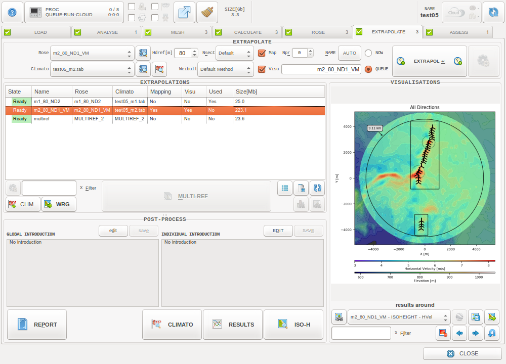
风数据外推选项卡
风速外推进程将选中的风数据应用于上一步生成的定向插值结果,根据插值结果和插值来源位置的风数据外推出整个项目区域的风资源分布。
风速外推进程的结果将被用于下一步发电量估算的输入信息, 或者以.wrg 文件导出在其他软件中进行后处理。
此进程同时允许将多个测风塔的外推结果进行综合。
进程选项

参考点的插值结果和风数据
- 外推的过程的起始点,即数据来源测风塔
- 风数据需与数据来源测风塔对应
如果没有使用对应测风塔的风数据,外推结果将无法真实反映该区域风资源分布情况。

扇区数量
外推中使用的扇区数. 默认值 36, 可以通过修改 用户偏好 来改变`.

韦伯拟合方法
Defines the Weibull fitting method used in extrapolation process (cf. Weibull fitting). The default method is the Moments method, it can be modified from the 用户偏好.

绘图,可视化
- 勾选绘图时,软件将允许导出整个关心区域的风资源绘图 (wrg),并且可以在等高图窗口中查看整个区域的外推结果。
- 勾选可视化时, 软件将允许在等高图窗口中查看整个项目区域包含关心区域和周围区域。
注解
只有勾选插值中的选项时,此选项才会被激活。

参考高度
在一个给定的位置,方向会随着高度的变化而变化,所以我们在做结果可视化时要考虑到高度 ( 用户偏好 )。
多塔综合

此操作将合并来自不同测风塔的外推结果以降低对该区域风资源分布评估的不确定性。
该进程使用反向距离(到参考测风塔的距离,距离越大占比越小)权重法来获得综合的外推结果, 该方法来源于Shepard.
- 选择所有将要用于综合的外推结果。
- 点击多塔综合。
注解
- 最终用于综合的外推结果需要来自拥有良好该地区风数据代表性的测风塔。
- 该合并过程不可被重复。
- 用于合并的外推结果必须有相同的”Hvane” 和 “Nsect”选项。
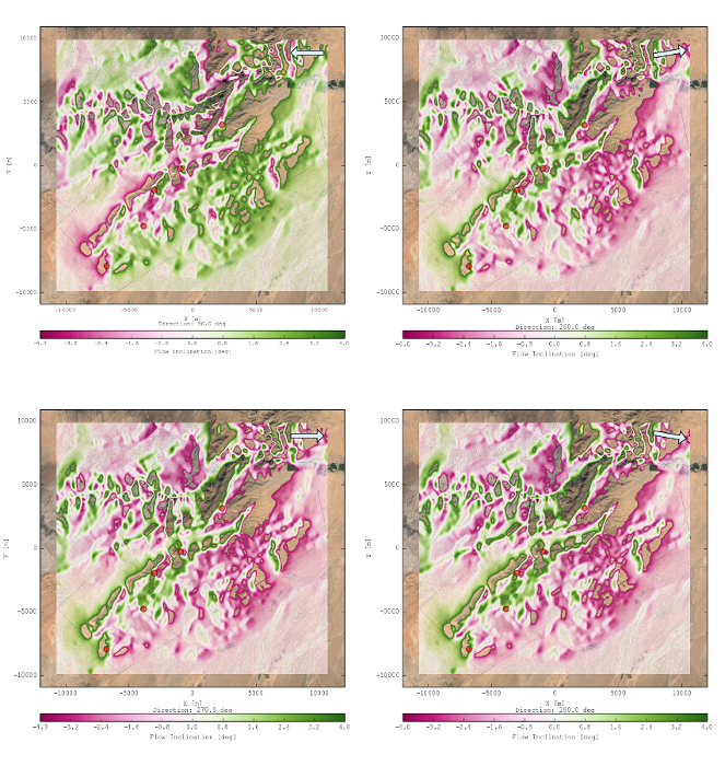
可视化
外推选型卡具有 等高图, Vertical Profiles,和 风能玫瑰图 可视化功能。
等高图按钮将允许在等高模式中查看外推的变量。可以查看的变量如下:
- 水平风速
- 入流角
- 湍流强度
- 韦伯尺度参数 - A
- 韦伯形状参数 - K
- Wind power density (cf. Wind power density)
风玫瑰图可观察的变量如下:
- 平均风速
- 风资源密度
- 入流角
- 绝对湍流强度
- 外推湍流强度
外推
气候

This button allows to export the extrapolated wind data at each entity into tab, WRG, or zsvd/zsvds format.
风力资源网格

This button allows to export gridded data files for each mapping entity into WRG or WRB format.
注解
To be able to export grid files, make sure to activate the Map option for the ROSE and EXTRAPOLATE processes.
WRG files
The conventional WRG format introduced by WAsP is a text file containing one header line, followed by one line per location considered, with the following information:
- X, Y坐标 [m]
- 地形海拔, WRG所在高度[m]
- Weibull parameters A [m/s] and k
- Wind Power Density [W/m2]
- Number of sectors considered
然后, 逐个考虑各扇区:
- 预测方向频率
- 方向性威布尔 A[m/s]和k参数
警告
尽管传统WRG被广泛使用, 它在用于发电量计算时候有着巨大的局限性, 由于把实际的风速简化成了威布尔参数, 它将不能总是保证方向性风速分布的准确性.
WRB files
The WRB format introduced by OpenWind is a binary file meant to address the lack of precision of WRG files. In addition to the information of a WRG file, it can include inflow angles, turbulence intensity, wind shear coefficients…
Please consult the OpenWind manual for the complete specifications of the WRB format.
技术说明
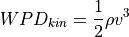
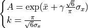
风资源密度
The formula for wind power density is usually derived from the classic wind power formula  ,
by simply normalizing it with the rotor area A, to get a density in W/m²:
,
by simply normalizing it with the rotor area A, to get a density in W/m²:
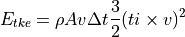
To take the Turbulent Kinetic Energy into account as well, we calculate the turbulent wind power density. The Turbulent Kinetic Energy is expressed as:
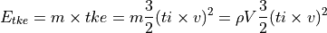
Now considering a small time  during which the air goes trhough a small volume of section A such that
  , we write:
Then dividing by time and section we get the turbulent wind power density:
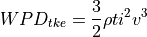
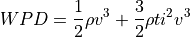
Which we add to the kinetic wind power density to get the total wind power density:
Weibull fitting
The statistical distribution most widely used to represent wind data is the 2-parameter Weibull distribution. Its Probability Density Function (PDF) and Cumulative Distribution Function (CDF) are defined as:
![f(v) = \frac{k}{A} \left(\frac{v}{A}\right)^{k-1} \exp\left[ -\left(\frac{v}{A}\right)^k \right] \\
F(v) = 1 - \exp\left[ -\left(\frac{v}{A}\right)^k \right]](../_images/math/160937637b67686ec347cc719902676ae75e97d9.png)
where  is the unitless shape parameter, and
  is the scale parameter in m/s.
To fit such a distribution from the extrapolation results, ZephyTOOLS implements 4 different methods:
- “Moments” -> Method of Moments
- “Least Squares” -> Least Squares Linear Regression
- “Max likelihood” -> Maximum Likelihood Estimation
- “Energy fitting” -> WAsP Method
Moments
The Method of Moments consists in equating the first 2 sample moments found in the data to the corresponding 2 population moments expected.
The obtained system of 2 equations allows to solve for the 2 parameters  .
.
The  population moment
  of the Weibull distribution is given by:
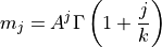
Where  is the gamma function.
The sample moment
is the gamma function.
The sample moment  of the data is computed as:
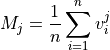
And as such,  (i.e. the data mean).
By equating
(i.e. the data mean).
By equating  and
and  we obtain the system:
This system has no analytical solution for  and would have to be solved numerically.
ZephyTOOLS instead considers the log-transformed data, taking  .
The obtained data follows a type-I minimum distribution
(better known as minimum Gumbel distribution, or log-Weibull distribution).
Its PDF and CDF are defined as:
.
The obtained data follows a type-I minimum distribution
(better known as minimum Gumbel distribution, or log-Weibull distribution).
Its PDF and CDF are defined as:
![g(x) = \frac{1}{\beta} \exp\left[ \frac{x-\mu}{\beta} \exp \left( \frac{x-\mu}{\beta} \right) \right] \\
G(x) = 1 - \exp\left[ -\exp\left(\frac{x-\mu}{\beta}\right) \right]](../_images/math/bc79d7b7f79961ac81a4c7c8cdd0453395592af8.png)
With:

While the method of moments on the original Weibull distribution has no analytical solution,
when using the log-Weibull distribution it can give estimators for the mean  and the standard deviation
  :
:
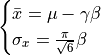
Where  is the Euler-Mascheroni constant.
So, the Weibull parameters can be estimated with:
is the Euler-Mascheroni constant.
So, the Weibull parameters can be estimated with:
Least Squares
The Linear Least Squares regression can be used on the Weibull CDF when rearranged as:
![\ln \left[ -\ln \left(1-F(v)\right) \right] = k\ln v - k\ln A](../_images/math/5eb6fa5d50d6b6caca4f9617237efeb9c472999c.png)
Which corresponds to a linear function  with:
with:
![\begin{cases}
y = \ln \left[ -\ln \left(1-F(v)\right) \right] \\
x = \ln v
\end{cases}](../_images/math/dd43b026dd72a2251159889035436151a936f3e3.png)
Where  is known from the frequency matrix of the data.
The parameters
is known from the frequency matrix of the data.
The parameters  and
and  are estimated with the Linear Least Squares regression as:
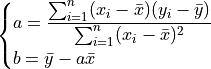
Finally the Weibull parameters are found with:
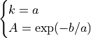
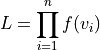
Max Likelihood
The Maximum Likelihood Estimation finds the Weibull parameters which maximize the statistical likelihood of the available data. The likelihood function is a product of the PDF functions, with one element for each data point in the data set:
It is mathematically easier to manipulate this function by first taking the logarithm of it. This log-likelihood function then has the form:
The log-likelihood function is computed for several pairs of parameters .
Initially combinations from coarse ranges of A and k values are tested, and the combination which returns the highest likelihood is taken as a first estimation.
Then the software tests iteratively several new ranges of values, each time with a finer step and always centered around the last estimation of .
This process allows to quickly assess with a precision of  for both.
Energy fitting
An implementation of WAsP’s method for Weibull fitting.
This method consists in finding the parameters which fill two conditions:
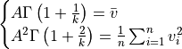
- The mean of the cubed wind speed of the fitted distribution is equal to that of the data. This comes down to equating the expected third moment to the corresponding third moment found in the data, much like what is done in the method of moments:
- The fitted distribution’s probability of winds above the data’s mean wind speed is equal to the proportion of the data meeting this requirement.
If we call this proportion
 we can express the condition as:
![1 - F(\bar{v}) = P_{v_i>\bar{v}} \\
\Leftrightarrow \exp\left[ -\left(\frac{\bar{v}}{A}\right)^k \right] = P_{v_i>\bar{v}}](../_images/math/e50746cd94ae8eebe7e8485a2276266e8620f1f8.png)
Finally,  can be subsituted using the first equation to get a single expression:
![\exp\left[ -\left( \bar{v}/\left(\frac{\overline{v^3}}{\Gamma \left(1+\frac{3}{k}\right)}\right)^{1/3} \right)^k \right] = P_{v_i>\bar{v}}](../_images/math/d78bcefdb3fddb0b0bb881de4c08db97d64a6f4a.png)
The left part of the equation is computed for several values of .
Initially a coarse range of k values is tested, from low to high until the first value allowing to meet the requirement is found.
Then the software tests iteratively several new ranges of , each time with a finer step and always centered around the last found acceptable value.
This process allows to quickly assess with a precision of .
Once is set, is calculated by solving the first condition’s equation.
IEC适用性
ZephyCFD提供了在每个涡轮机位置执行IEC站点适用性分析的所有工具:
- 平均风切变
- 最大风切变
- 最大风切变扇区
- 绝对倾角
- 最大倾角
- 最大倾角的扇形
- 全扇区15 m / s湍流强度
- 全扇形阵风湍流强度
- 全扇区有效湍流强度
- 全扇形有效阵风湍流强度
我们还将为每个涡轮机单独提供一个IEC矩阵,该矩阵将指示每个定向箱和每个风速箱是否适用于给定的IEC类别和类型的IEC。 生成的矩阵可用于有效地实施扇区管理。
布局优化
ZephyCFD导出的形状文件可用作简单约束(内部/外部)以执行布局优化。