ASSESS Tab
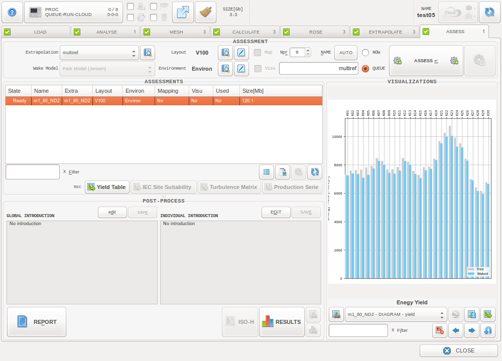
The ASSESS Tab
The ASSESS Tab is meant to perform a yield assessment using extrapolation results from the EXTRAPOLATE Tab, and considering wake effects: The turbines absorb the energy contained in the wind and create wakes downstream of the rotors. One of the observed effects in the wake zone is the reduction of the wind speed. These wake effects are transported by the wind flow, and can then affect the wind energy captured by other machines downstream.
ZephyTOOLS extracts the Annual Energy Production (AEP) and other related results at each wind turbine based on user-defined parameters such as turbine models and ambient details.
Process options

Extrapolation File
Use the result from the EXTRAPOLATE process as the input of assessment.

Wake Model
Currently it is only possible to calculate the AEP without wake model or with Park Jensen wake model. This feature is meant to help users get fast but less accurate results of AEP. In the near future, Zephy-Science will integrate Actuator Disc feature to directly consider the wake effects in CFD calculations.

Wind Turbine Models
The user have to associate .wtg files to the project’s wind turbines. It is possible to either set a single power curve for the whole farm, or to differentiate the turbine groups, or even each turbine individually.

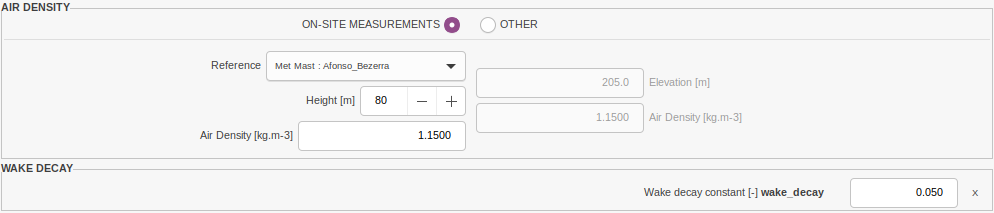
Environmental Parameters
The air density is considered constant. It can be set to a general value or a on-site value. The wake decay constant to use can be set here.

Mapping, Visualisation features
When Map is checked, the ISO-H visualizations are activated for the mapping areas.
When Visu is checked, the ISO-H visualizations are activated for the entire projected area.
Note
These options are only available if they were activated for the selected Extrapolation.
Visualizations
The EXTRAPOLATE Tab features Maps & Iso-Heights and Diagrams visualizations.
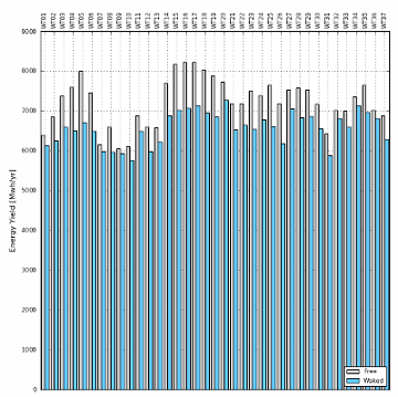
Click on the Results button to generate a bar graph showing the AEP for each wind turbine, with and without wakes.
Exportations
Yield Table

Exports a *.csv result file including Annual Energy Productions, wind speeds, and uncertainties for each wind turbine and for the farm as a whole.
Given the AEP information, users can obtain long-term production exceedance levels by defining:
- The losses as defined by MEASNET specifications.
- Historical uncertainties and inter-annual variation.
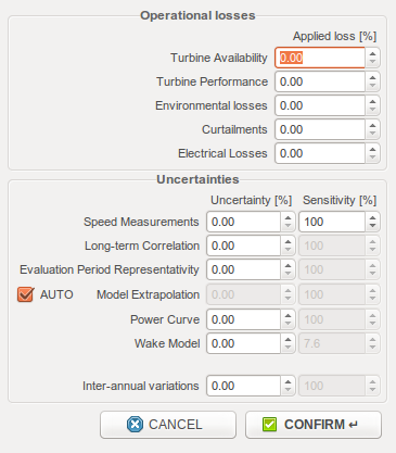
For historical uncertainties, the wind speed uncertainties should be weighted with the production model’s sensitivity to wind speed, hence the “sensitivity” variable. The wake model uncertainty sensitivity coefficient corresponds to the wake losses, as estimated by ZephyTOOLS.
By ticking “AUTO” on the model extrapolation uncertainty row, users can even quantify Turbine-wise uncertainties and find out the exact P50, P75 and P90 of each turbine.
In the exported .csv file, the first table gives for each turbine:
- Project name and Turbine Label
- Turbine Type and Capacity in MW
- X and Y coordinates [m]
- Terrain elevation, Hub Height [m]
- Free and Waked Mean Wind Speed [m/s]
- Wake Loss [%]
- Capacity Factor [%]
- Equivalent Hour [h]
- Distance to Nearest Turbine [m]
- Nearest Turbine Label
- reference height [m]
- Air Density [kg/m3]
- Power Density [W/m2]
- Average and Maximum Shear
- Direction of Maximum Shear [degree]
- Average and Maximum Absolute Inclination [degree]
- Direction of Maximum Absolute Inclination [degree]
- Weibull A [m/s] and k
The second table gives the Turbine-Wise uncertainties and productions:
- Gross, Array and Net Production [Mwh/yr]
- Nearest reference horizontal distance [km]
- Nearest reference vertical distance [m]
- Model Extrapolation Uncertainty (Base) [%]
- Model Extrapolation Uncertainty (Add) [%]
- Total Uncertainty [%]
- P75 Production [Mwh/yr]
- P90 Production [Mwh/yr]
- P95 Production [Mwh/yr]
Then the input losses and uncertainties are summarized. Finally the last table gives some global results for the complete site, for 1 year, 10 years and 20 years horizons:
- Future uncertainty [%]
- Total uncertainty [%]
- P50 Production [Mwh/yr]
- P75 Production [Mwh/yr]
- P90 Production [Mwh/yr]
- P95 Production [Mwh/yr]
Warning
The current version of the AEP calculation uses frequency matrix representations of the data. Hence, it cannot represent curtailment strategies which use hysteresis behavior: The LowSpeedCutIn and HighSpeedCutIn values given in the wtg file will be considered to be the same as the LowSpeedcutOut and highSpeedCutOut values, respectively.
IEC Suitability

Exports the evaluated wind conditions compatibility levels with the latest IEC standards.
This exportation is only available if the reference climatology of the used extrapolation includes a column of wind speed standard deviations.
In the exported .csv file, the first table gives for each turbine:
- Turbine Label
- X and Y coordinates [m]
- Terrain elevation, Hub Height [m]
- Weibull A [m/s] and k
- Air density [kg/m3]
- Average and Maximum shear
- Direction of Maximum Shear [degree]
- Average and Maximum Absolute Inclination [degree]
- Direction of Maximum Absolute Inclination [degree]
- Iref-15m/s(IEC-2016-dev)
- Iref-15m/s(IEC-2005)
- Iref-15m/s(IEC-1999)
The representative turbulence intensity value has different definitions in each IEC standard, but all the definitions are expressed using the same principle of combining the turbulence intensity mean and standard deviation:
- In IEC 61400-1 2016 edition, the quantile value at 70% is considered for classification, equation:
 .
. - In IEC 61400-1 2005 edition (Section 6.2 Table 1), it is the expected value of the turbulence intensity at 15 m/s:
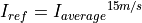 .
. - In IEC 61400-1 1999 edition, the value of average turbulence intensity plus standard deviation is the indicator for classification, equation:
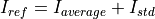 .
.
Furthermore, the .csv file includes a second table with turbulence standard deviation values by speed bins for each turbine, which also considers the wake effects.
These values are site-specific 90% quantile values (IEC 61400-1 Ed.3, Section 11.9, Equation 34),expressed as:  .
.
Turbulence Matrix

Exports a text file with the turbulence matrixes of a specific turbine.
The file starts with some turbine-specific information, namely:
- Turbine Label
- X and Y coordinates [m]
- Terrain elevation, Hub Height [m]
- Free and Waked Mean Wind Speed [m/s]
- Weibull A [m/s] and k
- Free Wind and Waked Wind sector frequencies
- Sector Wind shears
- Average and Maximum Shear
- Direction of Maximum Shear [degree]
- Frequency of Maximum Shear direction [%]
- Sector Wind Inclinations [degree]
- Average and Maximum Absolute Inclination [degree]
- Direction of Maximum Absolute Inclination [degree]
- Frequency of Maximum Absolute Inclination direction [%]
Then 3 tables give the turbulence mean, turbulence standard deviation and wake added turbulence, each discretized in bins of wind speeds and wind directions.
Time Series

Exports a text file containing time series of wind speed, wind direction, and gross energy production for a specific wind turbine.
Warning
The current version of this function will assess production values using freestream wind speed series. Hence, no wake model is applied, only the gross yield is considered.
Technical notes
PARK JENSEN Wake Model
- PARK Wake Model was initially developed and transplanted to WaSP by JENSEN and his friends.
- It assumes that the wind flow dissipates instantly behind the wind turbines after passing the rotors.
- The initial dissipation of wind speed is decided by the thrust curve of the wind turbine and the current wind speed.
- The wind speed recovers linearly behind the rotor along with the distance from the rotor.
- The speed of recovery depends on “wake dissipating index”.
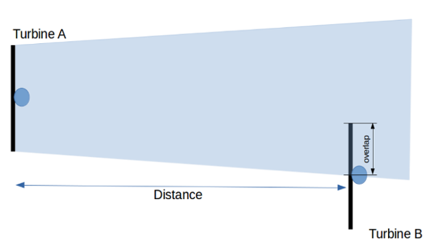
The dissipation of the downstream wind turbine can be calculated with the equation below:
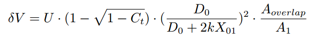
Where:
- U = Wind speed of upstream wind turbine at position A
- Ct = Thrust coefficient of upstream wind turbine at current wind speed
- X01 = Distance between WTa and WTb
- D0 = Diameter of the rotor
- k = Wake dissipating index
- Aoverlap = coinsided swipping area of wake from wind turbine A and the downstream rotor
The wind speed reaches wind turbine B equals to the free stream wind speed minus the wake loss result from the calculation above.
If wind turbine B is affected by multiple upstream wind turbines, only the maximum loss is considered.
Actuator Disc Wake Model
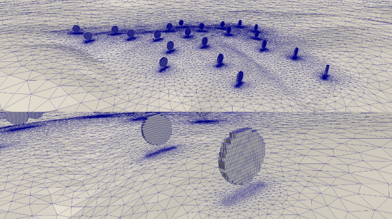
The meaning of introducing Actuator Disc Wake Model can be briefly explained as directly calculating the wake in CFD model, and taking the details missing in linear wake models into consideration (for example the wake effects from multiple wind turbines).
Currently the approach faces two big challenges:
- Mesh Refinement: To integrate wind turbine rotors in the CFD calculation, one needs to refine the rotor zone into 1m resolution. If using structured mesher which extends the refined zone to the boundaries, the number of cells will get to unimaginable amount.
- Calculation Power: Whatever structured or unstructured mesh is used for actuator disc model, very powerful hardware is required. This creates an impossible mission for the limited local hardware to generate the results in short duration.
It is clear that the root cause of not performing actuator disc wake model on general projects is the shortage of calculation power!
The Actuator Disc Process by Zephy-Science:
- ‘No Wake’ calculations run for 36 ten-degrees wind sectors
- Resulting wind directions are extracted at each hub location
- 36 actuator disk meshes are generated with the exact orientation of each rotors
- Flow is automatically initialized, considering a high wind condition thrust coefficient
- 10 consecutive CFD runs are processed
Between each process, the thrust coefficient is varied to evaluate the wake deficits for 10 different bins of wind speed. All speed bins and directions sectors are statistically processed with measurements
Note
Total: 38 meshes - 432 CFD computations - 37 remapping processes
Air density
How does ZephyCFD handle changes in air density?
There are two sort of variations:
Space-related variations
How density variations regarding the result locations are taken into account.
A reference air density ρref associated with a reference altitude href are specified as an input for the assessment process.
ρref: reference density in kg/m3
href reference altitude in m
These inputs are used to evaluate the density ρ at each result point, considering its altitude h in meters, following:
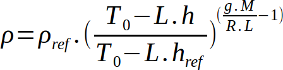
With:
- P0 = 101.325 kPa (sea level standard atmospheric pressure)
- T0 = 288.15 K (sea level standard temperature)
- g = 9.80665 m/s2 (earth-surface gravitational acceleration)
- L = 0.0065 K/m (temperature lapse rate)
- R = 8.31447 J/(mol.K) (ideal gas constant)
- M = 0.0289644 kg/mol (molar mass of dry air)
Time-related variations
How density variations regarding time are taken into account.
As in all other software, ZephyCFD Assessment Process does not take into account the variability of the air density over the time.
Note
This issue should be quickly tackled as it may drastically affect the energy estimation.
Turbine-wise uncertainties
The concept “turbine-wise uncertainty” is first introduced in version 18.09 to specify P75, P90 and P95 results for each turbine.
This early version of the algorithm considers that the uncertainty on the modelled wind flow increases linearly with the distance to the closest reference point. The vertical and horizontal components of this distance are considered separately, with scaling coefficients of their own. The scaling coefficients are empirical, and different depending on the site complexity which is assessed by the ZIX indicator.
The final uncertainty for a given point is expressed as: 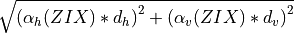
with  and
and  the horizontal and vertical distances respectively,
and
the horizontal and vertical distances respectively,
and  and
and  the scaling coefficients as follow:
| Complexity | ZIX | [%/km] |
[%/m] |
|---|---|---|---|
| simple | 0 | 0.5 | 0.05 |
| moderate | 1 | 0.7 | 0.07 |
| complex | 2 | 0.9 | 0.09 |
| highly complex | 3 | 1.0 | 0.1 |