MESH Tab

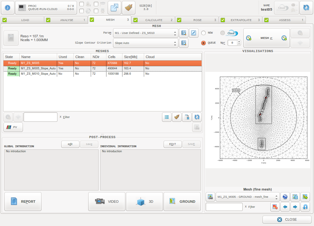
The MESH Tab

Before the numerical calculations, the 3D calculation domain needs to be discretized. This discretization process is also known as mesh generation, one of the most crucial steps in any CFD assessment.

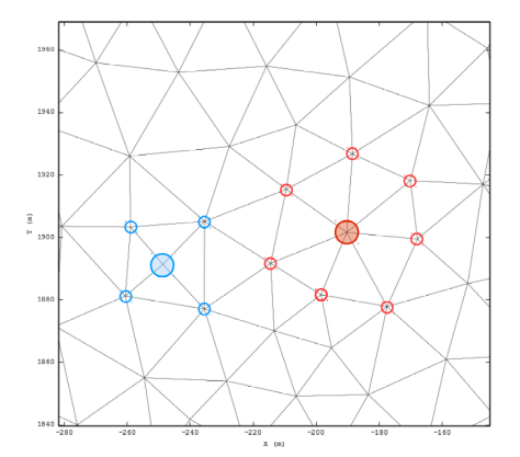
Traditional CFD tools use structured mesh techniques (cells are hexahedra) while ZephyCFD uses unstructured mesh techniques (cells are wedges: triangular prisms). The first figure below shows a 2D view of a structured mesh, the second figure shows an unstructured mesh used in ZephyCFD.

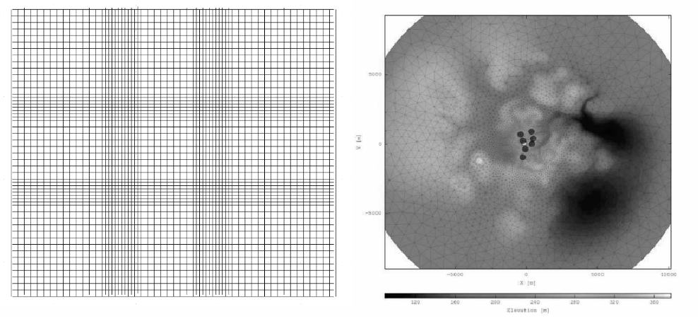
Refinement Zones of Structured Mesh and Unstructured Mesh

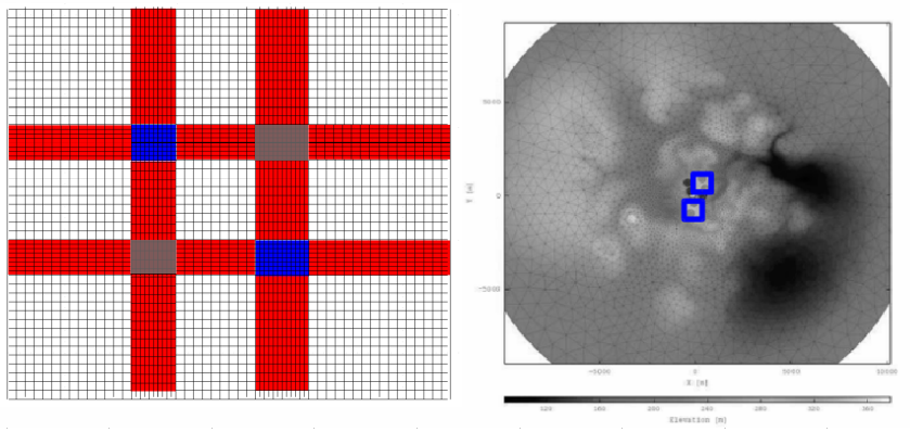
Refinement Strategy of Both Meshes

As we can see:

• Refinement “only-at-one-point” cannot be performed with structured mesh without affecting the refinement up to the calculation domain boundaries. This strong limitation doesn’t exist with unstructured meshes.
• With unstructured meshes, modelers have the flexibility to put more cells exactly where they are needed and less cells where they are not needed, which creates new opportunities for finer modeling : RIX-dependent meshes, Actuator Disk Wake Computations…

ZephyCFD uses a cylindrical mesh to simulate the wind flows in the project domain which can be used to calculate any directions just by rotating the boundary conditions around the outer domain boundary.

Cartesian meshes used in traditional CFD tools are forced to be perpendicular to the calculated wind direction and so one mesh is generated for each calculated direction.

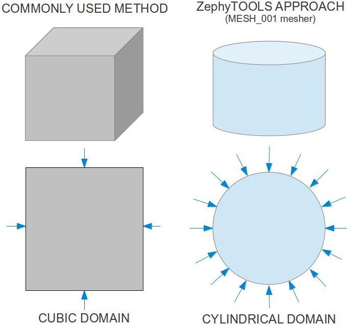
Comparison between Cubic and Cylindrical Calculation Domains

In ZephyCFD the domain is actually discretized twice:

• One COARSE mesh version: it is used uring the Initialization calculation
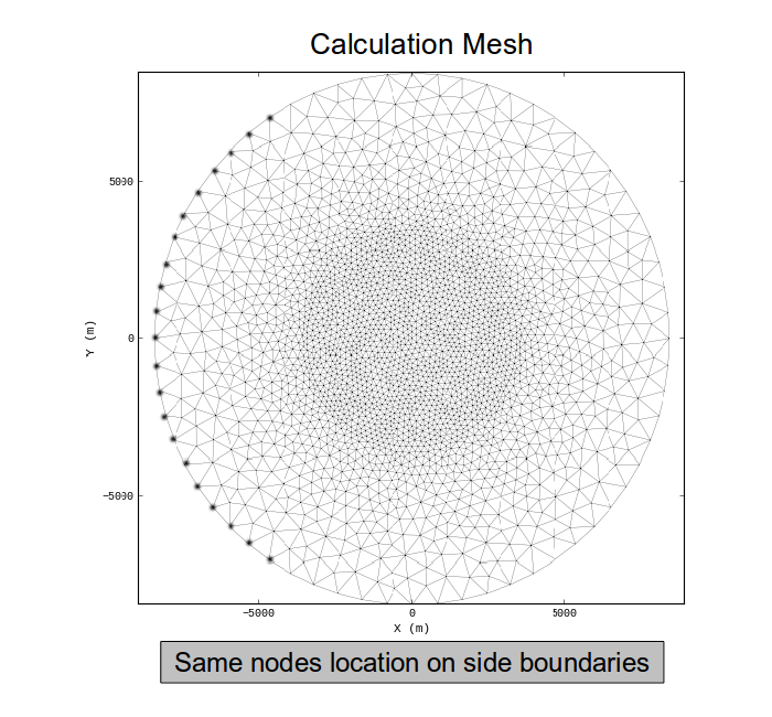
• One FINE mesh version: it is used uring the Final calculation

Note

The coarse mesh allows a ‘quick calculation’ to assess some relevent initial conditions for the fine mesh calculation. Less iterations are then needed for the final calculation to reach the convergence.

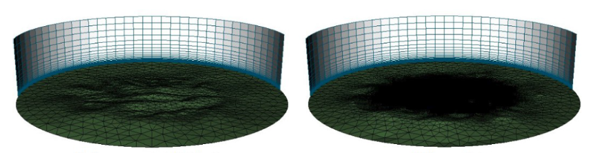
A new version of ZephyCFD will integrate Actuator Discs Wake Calculations (which refines the wind turbine rotor zones up to a 1-meter resolution). Integrating Wake calculations within the CFD simulations is crucial to consider, but not practically feasible with structured meshes as it would dramatically increase the number of cells…

Refined Wind Turbine Rotor in Actuator Discs Model

Process Options

Slope Contour Criterion: Select a slope contour to consider as area of interest when performing Heterogeneous Mesh Refinement. This can be defined from the Slope Contour definition window in the ANALYSE Tab.

Define the run type. For local types, define the number of processors to be used for the CFD simulations. Nproc 0 will automatically consider maximum available resource (=Total CPUs - 1).

Process Parameters

The parameters defining the Mesh process are read from the selected set of parameters.

The parameters can be divided in 3 groups

1. Horizontal Discretization Parameters
2. Vertical Discretization Parameters
3. Smoothing Parameters

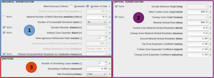
Horizontal Discretization

Users can decide to build a mesh based on a resolution target or a maximum number of cells.

The choice of the method depends on what should be prioritized : The resolution target will ensure a level of accuracy, while a maximum number of cells allows to control the calculation costs. Note that it is possible to quantify both the resolution and the number of cells before launching the process, with the “mesh preview” feature.

It is also possible to use either homogeneous refinement or heterogeneous refinement which will minimize cell consumption.

Consequently, several parameters are set automatically by default in order to:

• Decrease the effect of the side (inflow and outflow) and top boundaries
• Keep a good accuracy all over the zones of interest
• Keep a good robustness
• Taking the most advantage of the available hardware

All automatic parameters can be overwritten by the user if needed.

Note

resolution targets

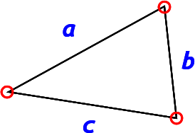
Horizontal resolution in wedges is not defined as in hexahedra:

Therefore the resolution parameters are driving the maximal distance between two nodes of a given cell.

Actually, the resulting resolutions may be finer than the targets:

The variation from parameter to resulting resolution is around 15%.

The parameters available for horizontal discretization are the following:

resfine

Refined Horizontal Mesh Resolution, in meters

Note

This parameter is only used when “Resolution” Mesh Accuracy Criterion is selected.

This directly specifies the maximal mesh resolution in Refined Zone Diameter, for the FINE mesh version.

Conditions

• 1 m < resfine < 500 m

meshlim

Maximal Number of Mesh Elements, in millions of cells

Note

This parameter is only used when “Number of cells” Mesh Accuracy Criterion is selected.

Drives the mesh resolution in Refined Zone Diameter, for the FINE mesh version, by evaluating the appropriate maximal mesh resolution to be applied, based on the specified Maximal Number of Mesh Elements.

Conditions

• 0.1 M < meshlim < 100 M

Automatic setting

• meshlim=-1 => Automatic setting is activated
• “meshlim” is then automatically evaluated from computer memory, with meshlim = TOTAL_RAM(Gb) - 1.e+6

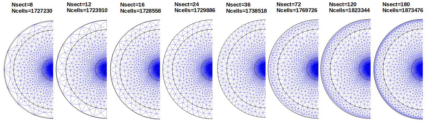
nsect

Number of Computable Directions

This defines the maximal number of computable directions. This parameter directly affects the horizontal resolution that will be applied near the domain boundaries.

Conditions

• nsect in [8,12,16,18,24,36,48,72]
• Directionnal step from 5 to 45 degrees

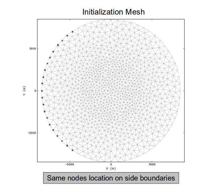
“nsect” leads to same sides discretization for both COARSE and FINE mesh versions.

Note

The higher the number of computable directions, the finer the mesh near the domain boundaries, and the higher will be the resulting number of cells.

To avoid unnecessarily high number of cells in areas which are not part of the domain of interest, a distance ratio set to 0.75 has been introduced, which defines a circle at 75% of the distance between the area of interest boundary and the boundary of the domain.

Within this area, the cells increase in size by a factor of 8 between the boundary of the area of interest and the circle defined by this ratio. Beyond this circle, the cells adapt their size to match the number of input directions (2 cells on boundary per input direction)

diadom

Domain Diameter, in meters.

Defines the circular zone over which the wind flow will be calculated.

Conditions

• diaref > diamin
• 11 km < diadom < 50 km

Automatic setting

• diadom=-1 => Automatic setting is activated
• The automatic setting will consider an extra distance of 10 000 meters around the Refined Zone Area

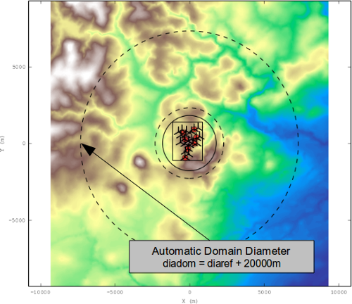
Domain Diameter: The wind is assessed over this circular area.

On the given example, the automatic setting is used for “diadom” (with 10 extra km from the Refined Area Zone).

diaref

Refined Zone Diameter, in meters.

Defines the central circular zone over which the “Refined Zone Horizontal Mesh Resolution” (“resfine”) will be applied.

Conditions

• diaref > diamin
• 1 km < diaref < 30 km

Note

The minimal diameter of a given project (“diamin”) is evaluated from the layout configuration.

It defines the circular surface (around the project’s centre) that fully covers the project’s entities, considering an extra distance of 50 meters around the entities.

Automatic setting

• diaref=-1 => Automatic setting is activated
• The automatic setting will consider an extra distance of 500 meters around the entities

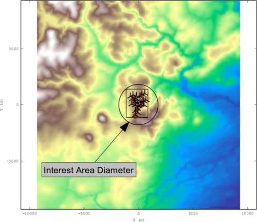
Interest Area Diameter: it defines the circle covering the whole layout.

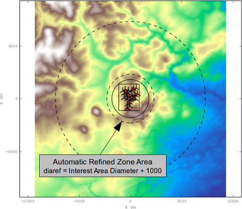
Refined Zone Area: The mesh is automatically refined over this surface of interest.

On the given example, the automatic setting is used for “diaref” (leading to an extra refinement distance of 500 meters).

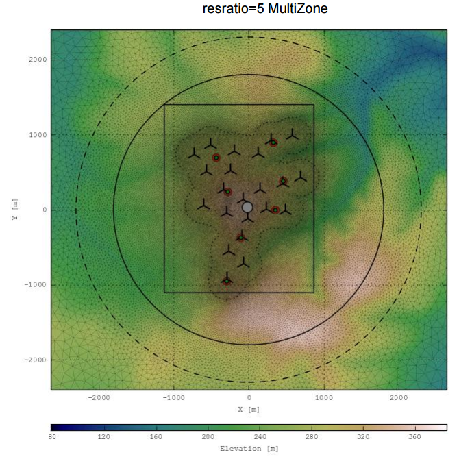
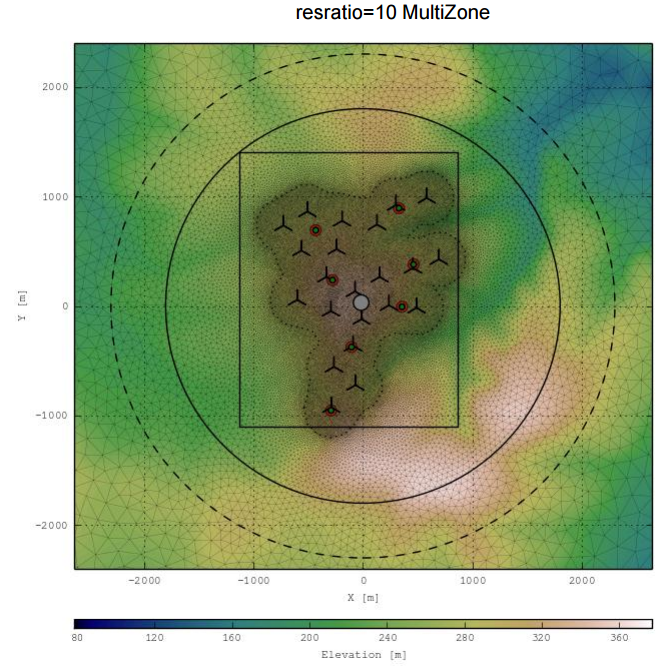
resratio

Heterogeneous Refinement Ratio

Conditions

• 1 <= resratio <= 10

Effects:

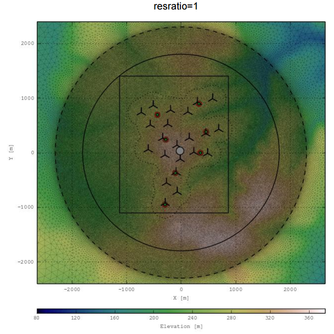
• resratio=1 => homogeneous refinement
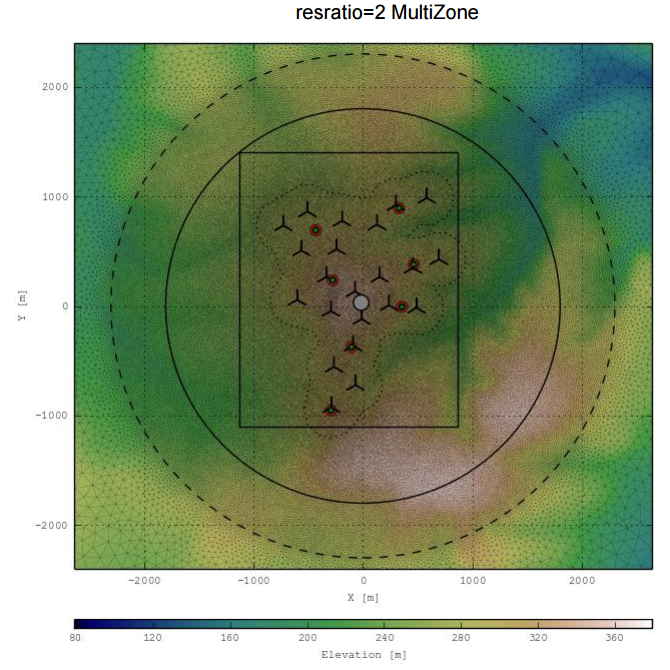
• resratio>1 => the heterogeneous refinement is activated: the Refined Horizontal Mesh Resolution is applied over the convex hull defined by all the mast/lidar/point/wt entities, considering an extra refinement distance equal to resdist.
• When resratio>1, the resolution is also controlled over Refined Zone Area by limiting the applied resolution to resratio × resfine.

Note

Check out the Technical Notes regarding heterogeneous meshing.

resdist

Heterogeneous Refinement Distance, in meters

Note

This parameter is only used when the heterogenous refinement is activated.

The heterogeneous refinement surface(s) is(are) generated considering this distance around each of the mast/lidar/point/wt entities.

Conditions

• 100 m <= resdist <= 500 m

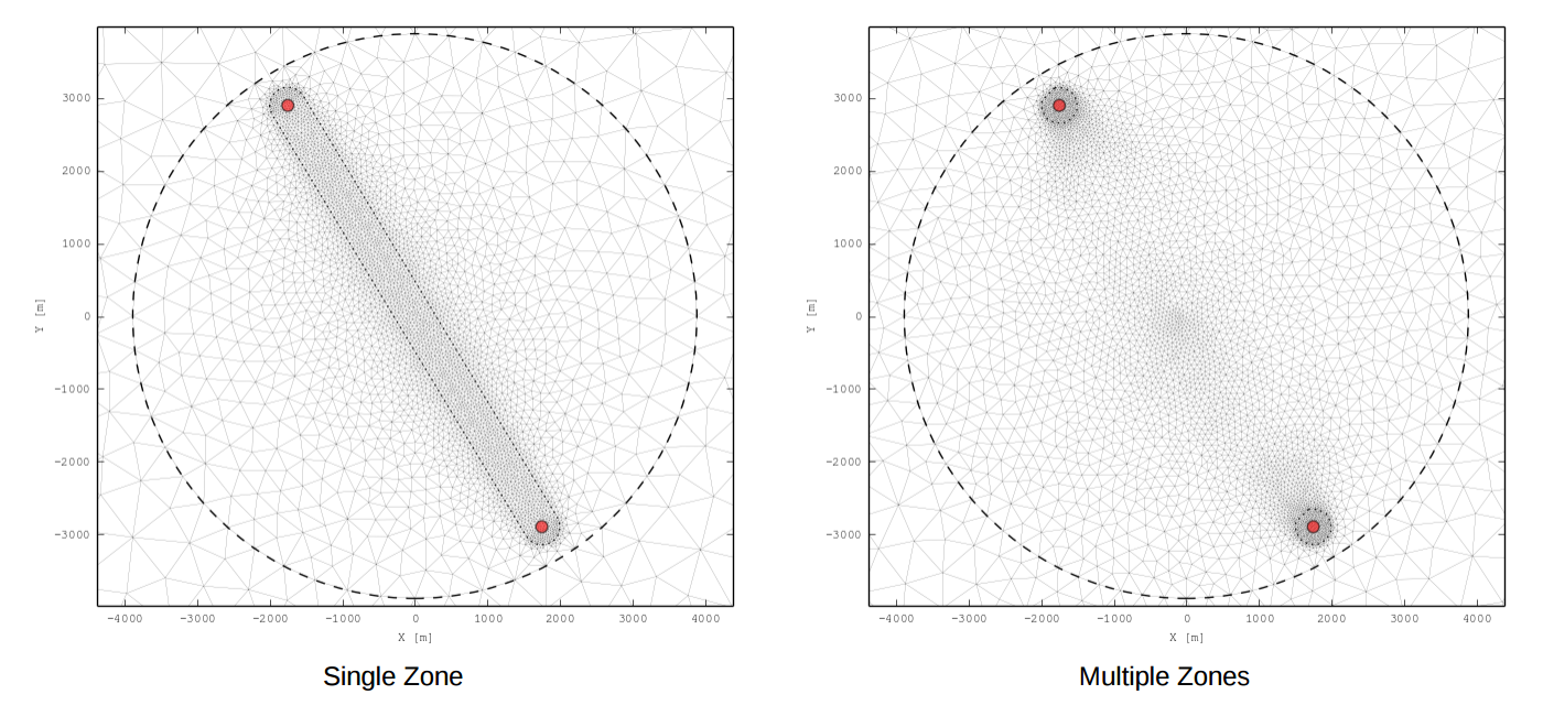
multizone

Multiple Refinement Zones

Note

This parameter is only used when the heterogenous refinement is activated.

A single surface can be generated, covering the whole refinement entities. It is also possible to generate for multiple refinement zones around the entities (around the group of entities when the corresponding surfaces are merged).

Conditions

• multizone in [‘Single Zone’,’Activated’]

Note

The “Single Zone” approach is mainly usefull for covering sparsed entities over a thin surface that should keep solved with accuracy.A typical case for using Single Zone approach would be a ridge with some sparsed masts over it, and with no other entity that would force the mesh to be refined over the complete ridge.

rescoa

Refined Horizontal Mesh Resolution for Initialization Calculation, in meters

This directly specifies the maximal mesh resolution in Refined Zone Diameter, for the COARSE mesh version.

Conditions

• 100 m < rescoa < 500 m

Automatic setting

• rescoa=-1 => Automatic setting is activated
• “rescoa” is then automatically evaluated using rescoa = 4 × resfine

Vertical Discretization

Control of the vertical size of the cells is defined over 3 different zones:

• Canopy zone
• Turbine zone
• Top zone

Why 3 zones ?

These 3 zones correspond to 3 areas of interest:

Elevation range [m]	0-10	10-150	150-2500
Cell size [m]	2-4	4-8	8-800
Interest areas	Ground obstacles	Wind turbines	Boundary layer

For each zone, 3 parameters are defined:

• Zone Height, in meters
• Maximal Vertical Resolution, in meters: cells size are limited with a maximum resolution over the zone
• Expansion Coefficient: cells height is increased by applying the specified geometric expansion coefficient

By default, ZephyCFD generates a set of pre-defined values, in order to:

• Decrease the effect of the top boundary
• Keep a good (robustness decreasing when vertical resolution decreases)
• Keep a good accuracy all over the rotors
• Keep a good accuracy all over the canopy volumes

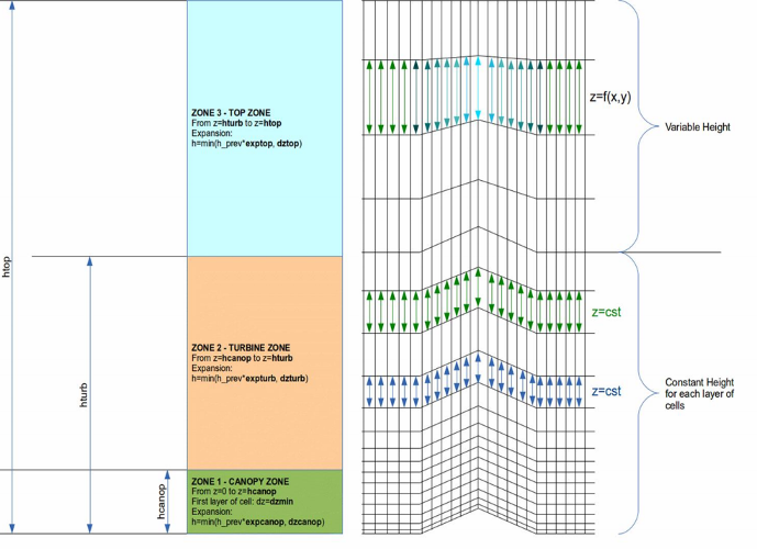
Top Zone

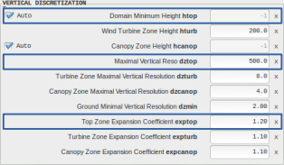
Domain Minimum Height: “htop”, in meters. Defines the height of the top boundary condition, regarding the lowest elevation data over the computation domain

Maximal Vertical Resolution: “dztop”, in meters

Top Zone Expansion Coefficient: “exptop”

Conditions

• 2500 m < htop < 10000 m
• 100 m <= dztop <= 1000 m
• 1 <= exptop <= 1.5

Automatic setting

• htop=-1 => Automatic setting is activated

The automatic setting will consider a project specific minimal height based on the orography variations, following:

Turbine Zone

Turbine Zone Height: “hturb”, in meters

Turbine Zone Maximal Vertical Resolution: “dzturb”, in meters

Turbine Zone Expansion Coefficient: “expturb”

Conditions

• 80 m <= hturb <= 500 m
• 5 m <= dzturb <= 20 m
• 1 <= expturb <= 1.5

Canopy Zone

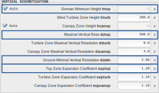
Canopy Zone Height: “hcanop”, in meters

Canopy Zone Maximal Vertical Resolution: “dzcanop”, in meters

Canopy Zone Expansion Coefficient: “expcanop”

Ground Minimal Vertical Resolution: “dzmin”, in meters

Conditions

• 0.01 m <= dzmin <= 2 m
• 10 m <= hcanop <= 80 m
• 2 m <= dzcanop <= 5 m
• 1 <= expcanop <= 1.5

Automatic setting

• hcanop=-1 => Automatic setting is activated

Canopy zone height is automatically evaluated, considering:

Note

Note: this parameter was mainly introduced to prepare for 3D canopy modelling, which is not available yet

Smoothing

There are different methodologies available for smoothing the terrain near the side boundaries.

General

Number of loops: “nsmoo”. Defines the number of smoothing loops to be performed over the ground mesh. The higher nsmoo will be, the higher the smoothing will be applied.

Coefficient: “smoocoef”. Defines how strong will be the smoothing in each of the smoothing loop. The higher smoocoef will be, the higher will be the applied smoothing.

Conditions

• 1 <= nsmoo <= 5
• 0 <= smoocoef <= 0.5

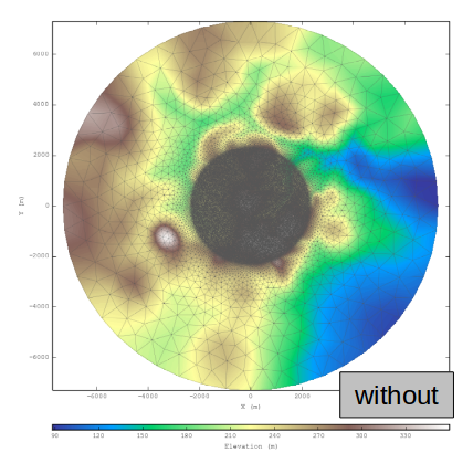
Inlet

“insmoo”

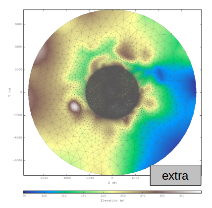
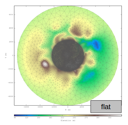
Defines the smoothing method near site boundaries of the domain.

Conditions

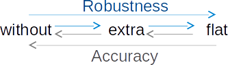
• insmoo in [‘without’, ‘extra’, ‘flat’]
• Option ‘without’: no specific smoothing is applied
• Option ‘extra’: the terrain near the side boundaries is smoothed
• Option ‘flat’: the terrain near the side boundaries is smoothed toward a flat terrain

Automatic Run

ZephyCFD offers to automate the meshing and calculation processes using the “Automatic Run” option. In this case the meshing parameters are chosen based on the ANALYSE results, and a set number of calculations are started in the CALCULATE section based on the climatology analysis.

Mesh Preview

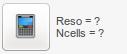
Once all the process options and parameters are set, before launching the process it is possible to calculate both the resolution and number of cells that you are about to generate. This is useful to choose an appropriate cloud configuration, or to check that your hardware can handle the size of the mesh.

Be careful that this process will freeze your GUI as it cannot be queued nor monitored. For heavy sites it may take a few minutes to complete.

Visualizations

The MESH Tab features Maps & Iso-Heights visualizations, and a specific 3D visualization module:

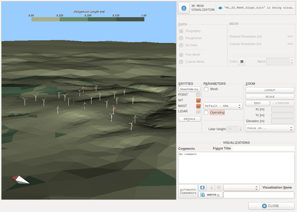
The 3D Mesh Visualization window

Storage optimization

In the “MESHES” frame, click this button to delete the main files related to the selected mesh, efficiently freeing space on your hard drive.

It is still possible to generate ground visualizations and reports of cleaned meshes.

Warning

Once a mesh is cleaned it is not possible to run calculations with it anymore.

Technical notes

An application of the Heterogeneous Mesh Refinement

Heterogeneous Mesh Refinement was introduced to minimize cell consumption by keeping a good accuracy.

On example given below, the Heterogeneous Refinement Ratio is varied, and the resulting Number of Cells is reported.

• Heterogeneous Refinement Ratio resratio varying from 1 to 10
• Constant Refined Horizontal Mesh Resolution: resfine = 10

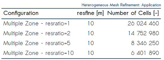
The other input parameters for the case are defined follow:

• Number of Computable Direction: nsect = 36
• Automatic Domain Diameter: diadom = -1
• Automatic Refined Zone Diameter: diaref = -1
• Refined Horizontal Mesh Resolution for Initialization: rescoa = -1
• Heterogeneous Refinement Distance: resdist = 250

Heterogeneous Mesh Refinement, when to activate it?

The choice of the method should be mainly linked with the calculation machine that will be used for running the calculations.

Evaluate first the need of accessing to finer resolutions that the “homogeneous method” is offering.

Depending on terrains and layout configurations, activating the Heterogeneous Refinement may sometimes lead to loose some important effects.

It is particularly suited in case of ridges.

Heterogeneous Mesh Refinement, an intermediate step to wake effects computations

Next ZephyTOOLS versions will include Wake Actuator Disk wake effect computations (CFD-based calculations of the wakes, particularly suited when wake-wake and wake-terrain interractions).

Catching the rotors with the mesh being particularly cells-consuming, the use of Heterogeneous Mesh Refinement is particularly suited (almost mandatory).

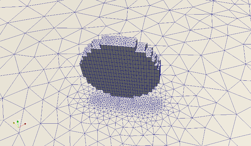
An example of a mesh catching the rotors volumes is given in next picture.

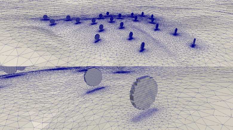
Heterogeneous Refinement enhanced to catch the rotors volumes and allow wake effects computations