CALCULATE Tab

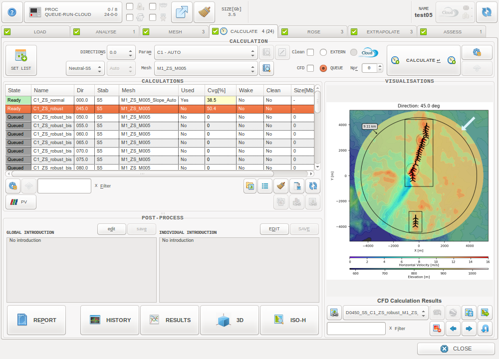
The CALCULATE Tab

Process options

Select the direction(s) for which CFD simulations will be run. This can be done either by:

• Selecting a single direction in the combobox.
• Selecting “Rose” in the combobox to automatically cover all the wind rose. It is possible to choose how many sectors to consider in the second combobox on the right.
• Setting an automatic or custom direction list from a dedicated interface accessible with the SET LIST button (cf. Direction List).

Select the mesh on which CFD simulations will be run. All the meshes generated for that project will be listed

Check “Clean” to automatically clean the calcultation when it is finished.

Check “CFD” to store additional CFD result variables: Velocity, vertical velocity, turbulent kinetic energy, turbulent dissipation rate, turbulent viscosity-pressure.

By default these options are deactivated, it is possible to modify the default behavior from the User preferences.

Define the run type. For local types, define the number of processors to be used for the CFD simulations. Nproc 0 will automatically consider maximum available resource (=Total CPUs - 1)

Direction List

From this window the user can define a List of Directions on which to launch calculations. By default, ZephyCFD tries to make an automatic selection. It is then possible to customize it.

Automatic selection

This automatic selection is performed only if the two default meshes (“ZS-Fine” and “ZS-Coarse”) have been generated. This can be achieved for example by using the Automatic Run option in the MESH Tab (cf. Automatic Run).

This is based on the input climatology analysis and chooses by default 52 directions: 26 on the fine mesh for predominant and highly-predominant directions, and 26 on the coarse mesh for non-predominant directions.

The predominant and non-predominant directions are defined by calculating the wind power density on 20°-wide sectors. Any direction within one of the four sectors with highest wind power density is considered predominant. For these predominant directions, the algorithm selects one every 4° to be calculated. Any direction within the other sectors is considered non-predominant. For these non-predominant directions, the algorithm selects one every 10° to be calculated.

The highly-predominant directions are defined by calculating the wind power density on 5°-wide sectors. Any direction within one of the four sectors with highest wind power density is considered highly-predominant. For these highly-predominant directions, the algorithm selects one every 2° to be calculated.

Custom selection

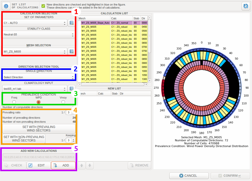
The SET LIST window

1. Basic settings for calculations (same as in the main window)
2. Single direction selection (same as in the main window)
3. Define prevalence condition by the directional distributions of “frequency of occurence”/”Wind power density”/”Average velocity”. At least one climatology file must have been loaded into the project to be able to use this.
4. Sort directions by wind prevalence, this will automatically add a list of directions in the box below.
5. Add list of directions to the “NEW LIST” on the right side, edit button will enable hand inputs.

The mesh used for the selected calculations is defined in mesh selection and is shown as the outer ring. Sectors in greed are selected directions, blue are added directions, and black are directions which have alreay been calculated. Changes of selected directions will be instantly visualized in the right picture.

Run type

It is possible to launch the calculation either locally, on ZephyCloud (cf. Configuration and Pricing) or on another machine (“extern” calculation).

Extern CFD Runs

Once the CALCULATE button is clicked with the “Extern” run type selected, Calculation Package folder(s) will be generated for each computable direction.

• Select the folder destination to export the Calculation Package folder(s).
• Copy the Calculation Package folder(s) on any of your external machine(s).

Note

Note: Only OpenFOAM needs to be installed on external machine(s) to run calculations.

To run calculation(s) on the external machine(s), open a terminal in the calculation folder and run the python command below:

python ZephyCLOUD_LAUNCHER_PROJECTNAME_np_X_nc_X_XXXXXXXXXX.py

Once each external run is completed, a result package will be stored in the same folder.

Go back to ZephyCFD CALCULATION tab and click on GET EXTERN to import your results.

Process Parameters

There are 4 predefined sets of parameters to tune the CFD Modeling Speed and Accuracy (Robustness-Convergence):

• Fast
• Robust
• Solid
• Simple

Fast, Robust and Solid parameters all use the SimpleC algorithm, enabling a significantly faster convergence, by a factor of 3 or 4 compared to the standard Simple solver. The simpleC algorithm needs much less relaxation (none for pressure, 0.9 for velocities and turbulence parameters).

In the main window, when selecting “AUTO”, ZephyCFD will automatically choose between the first 3 sets the one most suited to the site, according to the ZIX index found by terrain analysis.

“Robust” parameters will reduce divergence/innaccuracy risks but at the cost of computational time.

“Fast” should be used for relatively simple terrains without too many sharp contrasts, or simply if quick results are the priority.

“Solid” should be used for highly complex terrains. These parameters are those which reduce the divergence and inaccuracy risks the most, but they are the most expensive too, in terms of computational cost.

“Simple” is using the standard Simple algorithm (it corresponds to the previous Robust solver).

Check out Convergence Speed for an example of how these three solvers behave compared to one another.

More predefined solver parameters can be added to the list by defining them from the ZephyTOOLS Main Menu/Preferences/Default CFD User-Defined calculation parameters.

It is always possible to customize these sets of parameters with user defined solver settings, which can be of particular interest for experienced CFD users.

Solver Settings

Warning

Only for CFD experts

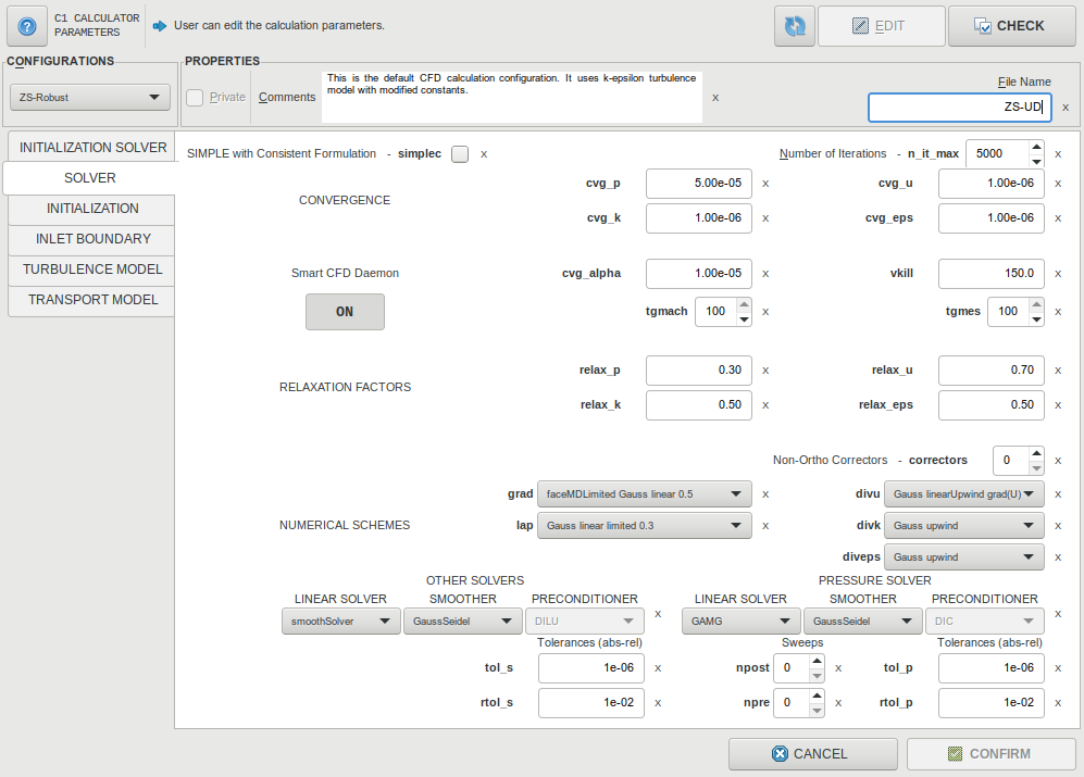
The CFD calculation parameters window

The solver settings for the initialization and main calculation are available in the first and second tabs.

Smart CFD Daemon

It is a tool introduced in version 19.07 designed to extend and improve on OpenFOAM’s built-in convergence criteria (residuals of pressure,velocity,k and epsilon). It can simply be switched on/off with a button in the user defined parameters, and is switched on by default for the predefined parameters.

Convergence is calculated for each defined wind turbine and measurement location (e.g. met mast or lidar) separately, and the daemon will stop the calculation once a set ratio of turbines (“tgmach”, in %) and measurement locations (“tgmes”, in %) meet the “cvg_alpha” criterion. By default, this ratio is 100% for both turbines and measurement locations.

In addition, the Smart CFD Daemon implements a simple safeguard to spot divergence in the calculations: If the horizontal wind velocity is detected to be higher than a predefined criterion “vkill” (default value of 150m/s) on any defined entity, the calculation will be killed.

Relaxation factors

The relaxation factor is another important parameter governing the stability of your results. Relaxation is used to stabilise calculations by mixing results from the current step with results from the previous step. A relaxation value of 1.0 completely ignores the previous step while a value of 0 implies that the results won’t change. Decreasing the relaxation factor can be a solution for unstable calculations, but this will come at the cost of increasing computation time.

The list of available numerical schemes are taken from OpenFOAM, and are discretisation schemes for the gradient, divergence and Laplacian terms in the steady-state incompressible Navier-Stokes equation. A detailed explanation for each term can be found on this page of the OpenFOAM user guide.

The different solver options for each variable are also taken from OpenFOAM. The paper (Behrens,2009) gives a good overview of the different linear solvers, preconditioners and smoothers offered by OpenFOAM and used in ZephyTOOLS.

Initialization Settings

Defines if an initialization calculation is run on the coarse mesh.

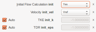
Inlet Boundary Conditions

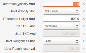
ZephyCFD uses a log wind profile as an input at the boundary. The default values are 30m/s wind speed at 500m height, with a roughness length taken from the local file/database value.

Turbulence Model

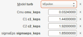
ZephyCFD currently proposes three different turbulence models:

• Standard k-epsilon
• RNG k-epsilon
• Realizable k-epsilon

The coefficients of the standard k-epsilon model are modified to take into account the atmospheric boundary layer (see Stevanovic et al., 2009, “Validation of atmospheric boundary layer turbulence model by on-site measurements”).

The RNG and realizable models are two other alternatives to represent turbulence in the ABL domain.

Convergence Monitoring

Click on the “Control” button to monitor the running CFD calculation and its convergence.

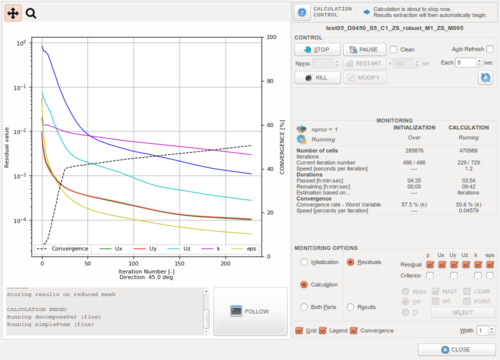
ZephyCFD Calculation Result Monitoring Window

ZephyCFD advocates fully transparent assessment processes. It supports reporting and exporting of the entire calculation process (inputs and results from all steps). Each process can be reproduced by any third-party which guarantees the reliability of the calculation.

In terms of convergence, ZephyCFD allows to monitor the convergence process in real time and add iterations to any simulation not fully converged.

This is done after observing the fluctuation of residual values as well as results (wind speed, TI, shear) at any selected points, which provides a fully-transparent picture of the CFD process.

• Residuals are the differences in results between the current iteration and the previous.
• CFD results (speed, TI, shear) at each entity location (WTG, mast, etc.) at each iteration.

Users can monitor both simulation behavior and reliability!

Note

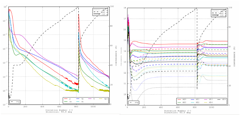
In previous versions, the global convergence indicator was based on residual values. Since version 19.07, the convergence criterion has been modified as it is now based on the standard deviation of Wind Shear results (alpha) for the last 50 iterations (10 registered values taken every 5 iterations). This standard deviation is compared with a predefined in-house convergence criterion, “cvg_alpha”. The global convergence is considered to be the one from the point of interest with the worst convergence.

This has been implemented to avoid unnecessary iterations if results have converged to stable values but residuals keep having a poor convergence due to small oscillations between iterations.

Note

Whenever 100% convergence is reached, Calculations will automatically be stopped. If results are stable, you can stop the run before 100% convergence rate is reached.

STOP Button

You can stop the process by clicking on the STOP button in the CONTROL frame. This will stop the process and save the results.

KILL Button

You can kill the process by clicking on KILL button in the CONTROL frame. This will kill the process without saving the results.

Refresh Buttons

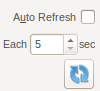
In addition to the manual refresh button, you can enable the Automatic Refresh and set the refresh time to monitor the convergence rate, residuals / results in real time.

PAUSE/RESTART Buttons

It is possible to PAUSE and RESTART a calculation as needed. The number of processors to use can be modified before restarting. In the case where the calculation has hit the maximum number of iterations, the user can choose how many additional iterations should be calculated.

Cloud Management

Note

Note: Check out Configuration and Pricing on how to set up and launch a cloud process.

Buttons with this symbol allow to download cloud calculation results. The one on the right of the “CALCULATE” button will download results from all the existing cloud calculations at once, while the one below the calculation list will only download the results of the selected calculation.

When clicked, a small window will pop up:

It is possible to select which kind of files should be downloaded, the main results being mandatory. The two other possible set of files may incur large downloads.

This button will delete the cloud version of the calculation from the ZephyCloud servers (cf. Storage Cost). Make sure to have retrieved your results before doing so.

Visualizations

The CALCULATE Tab features Maps & Iso-Heights, Vertical Profiles, and a specific 3D visualization module:

ZephyCFD allows to observe the CFD results in different 3D modes: Iso-height, sectional distribution and wind trajectory. The engineers can travel around in the 3D mode to gain more direct views of the result distributions.

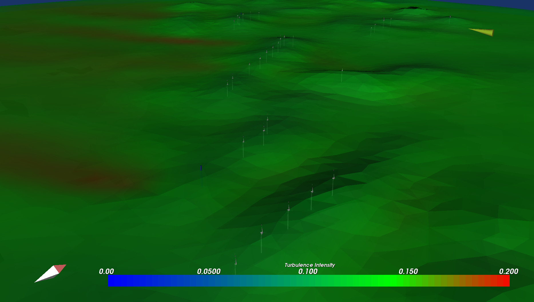
Turbulence Intensity in 3D Iso-height Mode

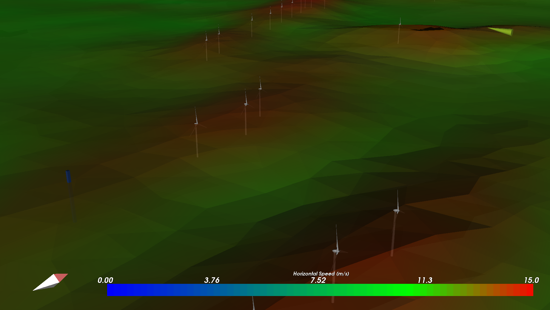
Horizontal Wind Speed in 3D Iso-height Mode

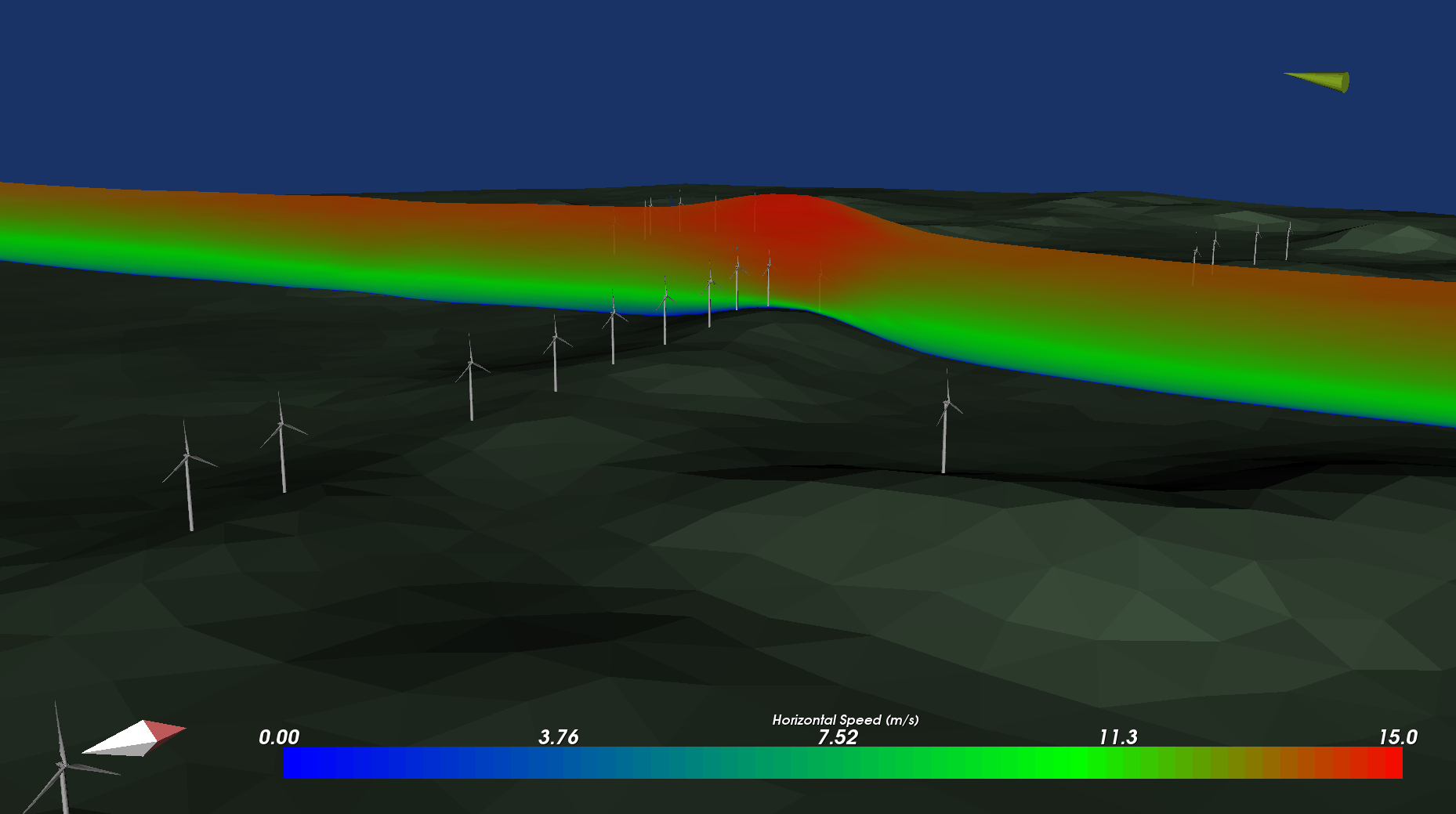
Horizontal Wind Speed in 3D Sectional Mode

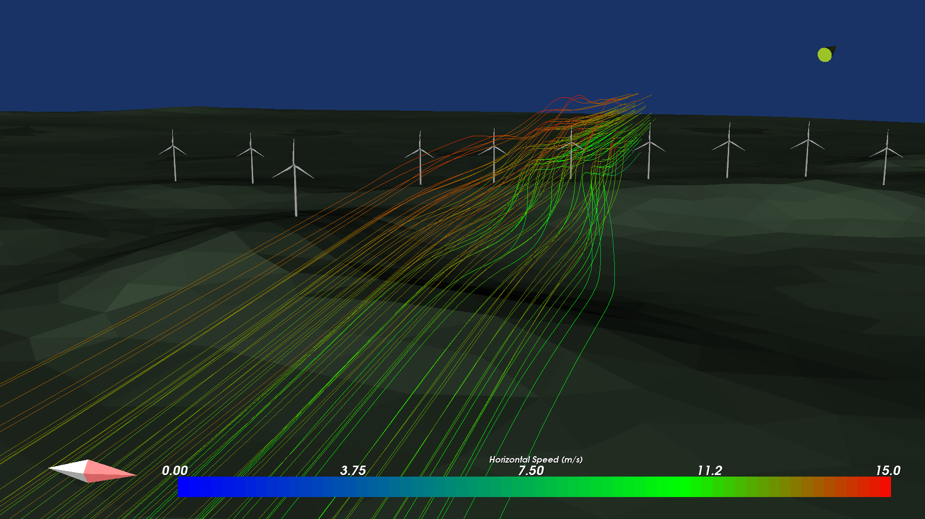
Horizontal Wind Speed in 3D Trajectory Mode

Storage optimization

In the “CALCULATIONS” frame, select one or several calculations and click this button to free some space on your hard drive.

A small window will pop up:

It is possible to delete either:

1. The files containing the necessary data to locally restart the calculation at the last iteration and/or open it in ParaView.
2. The stored result files necessary for the 3D visualizations and/or to post-extract the results (to modify the layout configuration).

You can keep track of which files have been deleted with the “Clean” flag of each calculation:

• “No” : All files are present
• “No restart”: option 1. has been used
• “No extract”: option 2. has been used
• “Clear”: options 1. and 2. have been used

It is still possible to generate roses, visualizations and reports from cleared calculations.

Technical notes

Turbulence Models

One Equation Vs. Two Equation?

Back in 2009, the famous Bolund wind flow simulation blind test showed that dual turbulence equation models have higher accuracy levels than single turbulence equation models (cf Part I, Part II ).

The figure below shows the results from Bolund TI model blind test. As we can see in the results table, 11 models in the the top twelve models were using dual turbulence equation models.

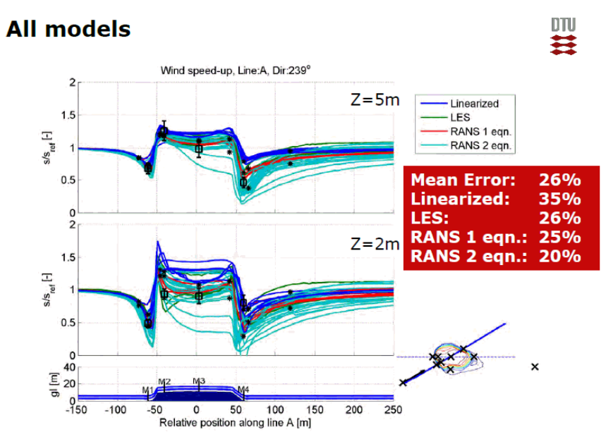
Average error of different turbulence models in the Bolund experiment

Top 10 ListID	Turb. model	Error [%]	Error 5m [%]
ID0053	RANS k-epsilon	13	6
ID0037	RANS k-epsilon	14	4
ID0000	RANS k-epsilon	14	5
ID0036	RANS k-epsilon	14	5
ID0016	RANS k-epsilon	14	5
ID0015	RANS k-epsilon	15	5
ID0077	RANS k-epsilon	15	5
ID0010	RANS k-epsilon	15	7
ID0009	RANS k-epsilon	15	5
ID0034	RANS 1 eqn.	17	7
ID0068	RANS k-epsilon	17	10
ID0006	RANS k-epsilon	17	6

Thermal stability

Currently ZephyCFD can only consider a neutral thermal stability, but our development team is working on the subject.

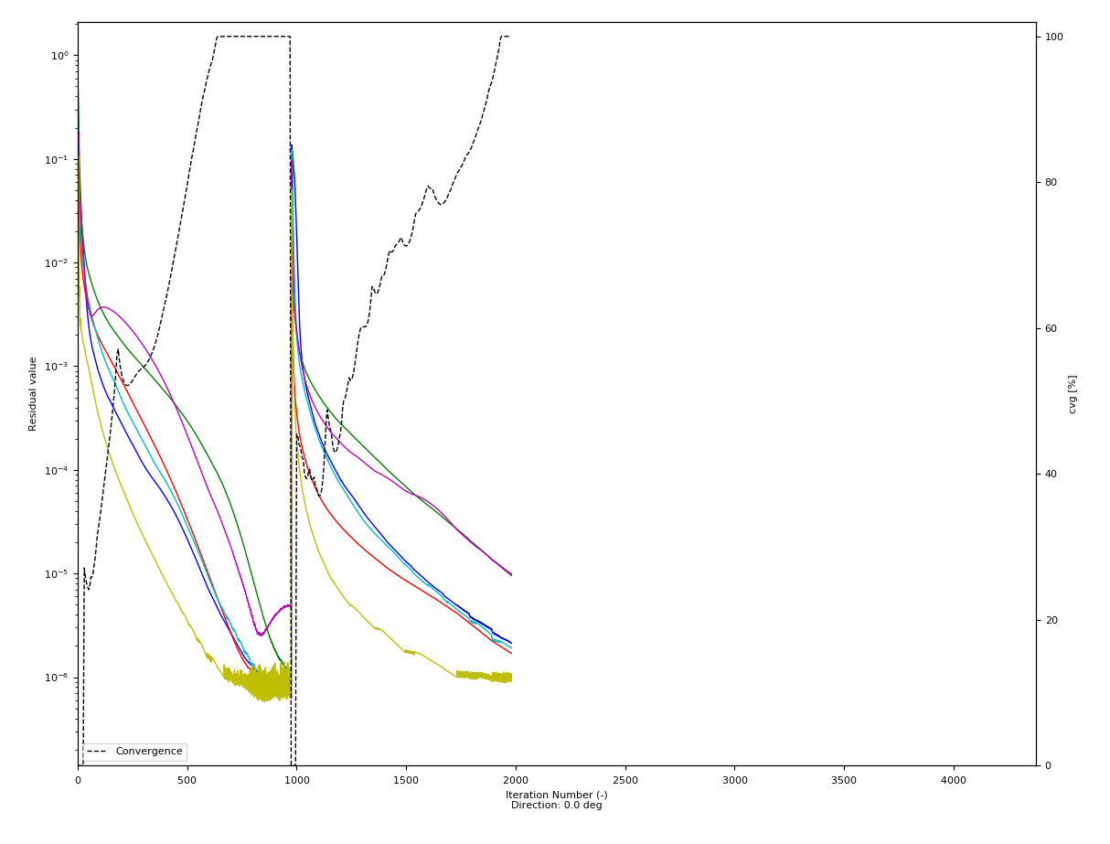
Convergence Speed

The calculation residuals obtained from the Fast, Robust, Solid and Simple solvers are compared below for the CREYAP site with a 2.2 million cell mesh and a synoptic wind direction at 0 degree. The x-axis goes to 4400 iterations and the convergence (in %) is represented by the black dashed line.

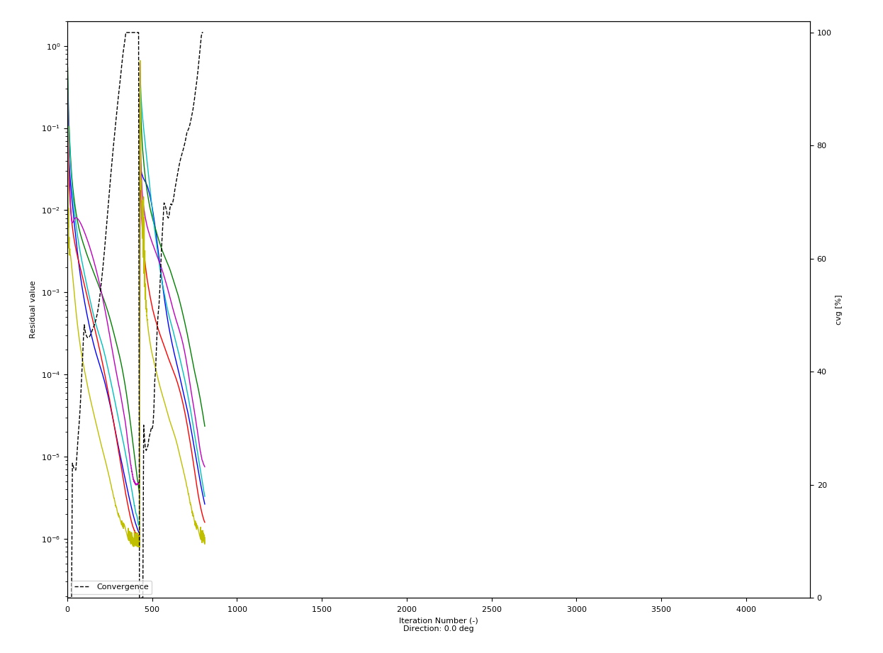
Calculation residuals with FAST parameters

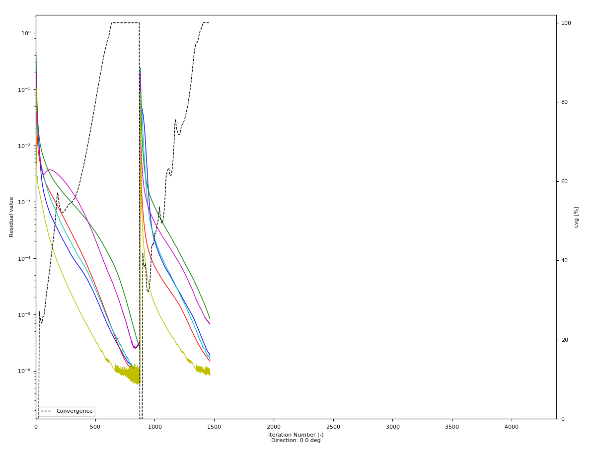
Calculation residuals with ROBUST parameters

Calculation residuals with SOLID parameters

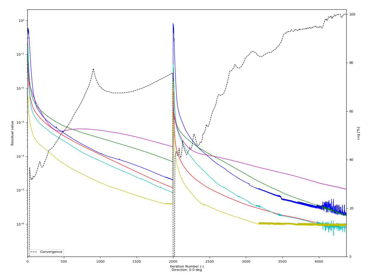
Calculation residuals with SIMPLE parameters

As the CREYAP site is not too complex, all solvers reach 100% convergence and calculations can clearly be optimised by choosing the faster solvers. Moreover, it can be observed that the calculations using the SimpleC parameters have highly better performance than the one using the Simple algorithm.